How to Create a Drop-Down List in Excel (2024)

Introduction

Drop-down lists in Excel are powerful tools for streamlining data entry and ensuring consistency in your spreadsheets. They provide a user-friendly way to select predefined options, saving time and minimizing errors. Whether you’re using Excel on Windows or Mac, creating drop-down lists is very easy task!

Preparing Your Data

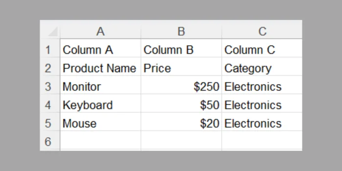
1. Gather your list entries: Compile the options you want to appear in your drop-down menu. These can be anything from product categories to project statuses and can be located in any column or sheet within your workbook.
2. Separate each entry: Ensure each option occupies a distinct cell. This structure is essential for creating the list source.

Create a Drop-Down List in Excel

1. Select target cells: Click on the cell(s) where you want the drop-down menu to appear. You can select multiple cells if you intend to use the same list across them.
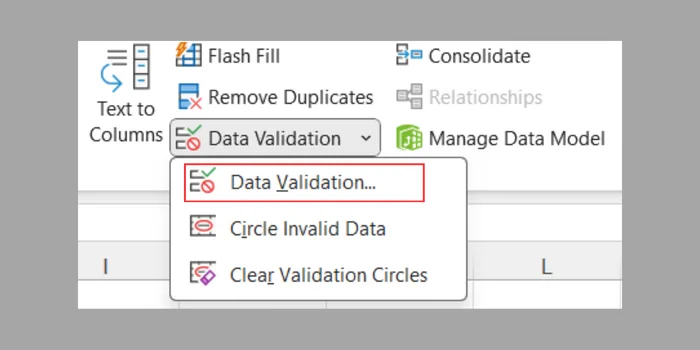
2. Access Data Validation: Navigate to the Data tab on the ribbon. Within the Data Tools section, locate the Data Validation button and click it.

Setting Up the Validation Rules

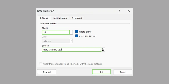
1. Choose “List” under “Allow”: In the Data Validation window, under the Allow section, select List from the drop-down menu. This specifies the type of validation you’re applying.
2. Define the data source: In the Source field, you have two options:
   • Directly type the list: Separate each entry with a comma, like High, Medium, Low.
   • Select the range: Click the small arrow next to the Source field and directly choose the range of cells containing your list entries in the spreadsheet.
3. Confirm your choices: Click OK to finalize the data validation process and save the changes.

Optional Customization (Windows Only)

This step is exclusive to the Windows version of Excel:

1. Right-click the cell: Access the context menu by right-clicking on the cell containing the drop-down list.
2. Select “Data Validation”: Choose Data Validation from the menu options.
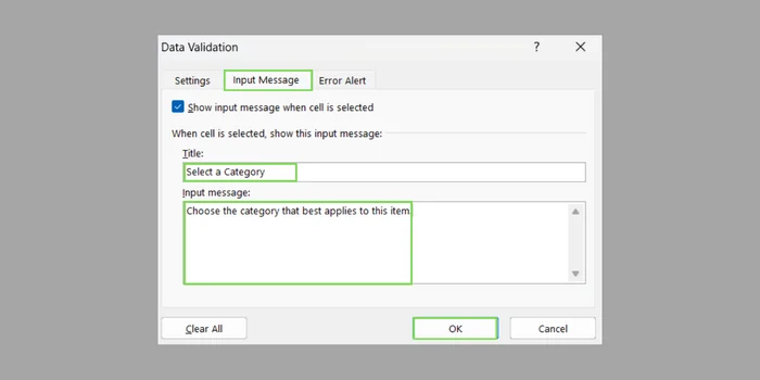
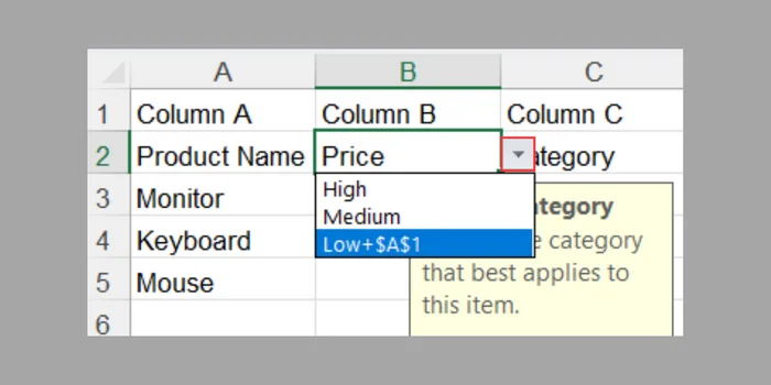
3. Customize the list (Input Message tab): Click the Input Message tab. Here, you can create a Title and Message that will appear when users hover their mouse over the cell. This adds clarity and guidance for list users.

Testing and Using Your List

1. Click the cell: Click on the cell with the newly created drop-down list.
2. Observe the arrow: A small arrow should appear on the right side of the cell, indicating the presence of the list.
3. Access the list: Click the arrow to reveal the list of options you defined earlier.
4. Make your selection: Choose the desired option from the displayed list.
5. Data is set: The selected option will instantly populate the cell, ensuring data consistency and clarity.

Remember

• You can modify the list entries by editing the data in the source range you specified during creation.
• For advanced users, creating a named range for your list entries and using it as the source is also possible.

By following these simple steps, you can effortlessly create and manage drop-down lists in your Excel spreadsheets on both Windows and Mac. This versatile tool enhances user experience, promotes data accuracy, and empowers you to build well-organized and efficient spreadsheets.

Additionally Microsoft 365 Basic is a new $1.99 a-month subscription with 100GB OneDrive and Ad-Free Outlook.