Introduction to Freezing Rows and Columns in Excel
When working with Microsoft Excel, the ability to freeze rows and columns in Excel comes in incredibly handy, particularly during data analysis and navigation. This feature essentially allows you to keep certain parts of your spreadsheet – usually headings or key data points – visible at all times as you scroll through your document.
It’s akin to having certain elements “stick” to the top or side of your viewing area, ensuring they remain in view no matter how far you scroll down or to the side. This functionality becomes a cornerstone for efficiency and ease of use in various data-handling scenarios.
Why do Freezing Rows and Columns Matter?
- Constant Visibility: By freezing rows or columns, crucial information remains in sight, eliminating the need to scroll back to the top or the side to remember which data you’re viewing. This is particularly useful for spreadsheets with extensive data.
- Simplified Data Comparison: Freezing panes make it easy to compare information across distant parts of your spreadsheet. This feature ensures that headings or key data points are always visible, facilitating quick comparisons without losing your place.
- Enhanced Navigation: With important data fixed in place, navigating through complex datasets becomes less cumbersome. You no longer have to worry about losing track of column or row headings, making data analysis more straightforward.
Ideal Scenarios for Freezing Panes
- Handling Large Datasets: Where your spreadsheet contains a significant data value, freezing rows or columns can help you maintain orientation and quickly access the necessary information.
- Creating Reports: For reports that require constant referencing of top rows or leftmost columns for data accuracy and context, freezing these sections can be extremely beneficial.
- Comparing Distant Data: When your analysis involves comparing figures or entries that are far apart, having key rows or columns frozen ensures that you can make accurate comparisons without the hassle of scrolling back and forth.
What Does “Freezing Panes” Mean?
In Excel, freezing panes is a feature that lets you keep specific rows or columns visible while you scroll through the rest of your spreadsheet. It’s like pinning these rows or columns in place, so they stay on your screen no matter how far you move up, down, or sideways.
How Freezing Panes Affects Data Navigation
- Stay Oriented: With titles or important data always visible, it’s easier to understand and work with your data. You won’t mix up columns or forget what each column represents.
- Scrolling Made Easy: You can scroll through lots of data without losing sight of your headings. This means you can compare numbers or entries from different parts of your spreadsheet without flipping back and forth.
The Difference Between Freezing Rows, Columns, and Both
- Freezing Rows: This keeps the top part of your spreadsheet fixed. For example, if you freeze the first row, your column titles will always be visible as you scroll down.
- Freezing Columns: This option locks the left side of your spreadsheet. If you freeze the first column, you’ll always see your row labels (like names or dates) as you scroll to the right.
- Freezing Both Rows and Columns: Excel also lets you freeze both rows and columns at the same time. This way, you can keep both your top headings and side labels in view, no matter where you navigate on your sheet.
Freezing panes in Excel is all about making your data easier to manage by keeping important information visible at all times. Whether you’re dealing with large datasets or need to maintain a clear view of your data structure, freezing panes can significantly enhance your navigation and analysis capabilities.
Preparing Your Excel Sheet for Freezing Panes
Before you use the freezing panes feature in Excel, organizing your spreadsheet properly can make a huge difference in how effective this tool can be. Here’s how you can prepare your Excel sheet for optimal results:
1. Place Headings at the Top
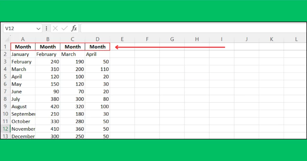
- Use the First Row: Your column headings should be in the first row of your spreadsheet. This makes it clear what each column represents when you freeze the top row.
- Clear and Concise: Make sure your headings are straightforward and understandable at a glance.
2. Sort Your Data
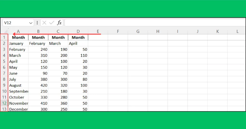
- Logical Order: Arrange your data in a way that makes sense for what you’re doing. For example, you might sort data alphabetically, by date, or by another relevant category.
- Consistency: Keep your sorting method consistent across the spreadsheet to avoid confusion.
3. Use Filters If Necessary
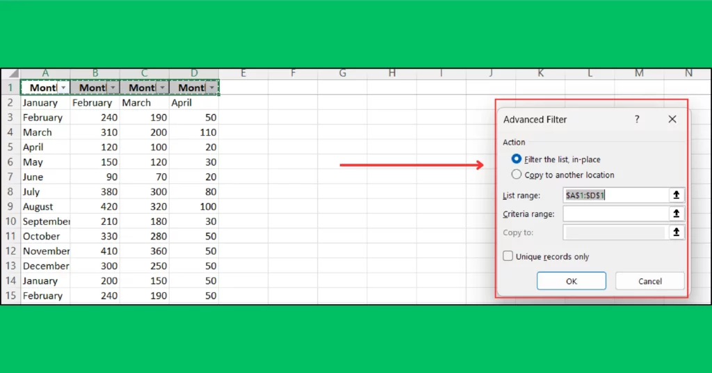
- Filters for Ease: Adding filters to your column headings (after freezing the top row) allows you to easily sort and filter through your data without losing sight of your headings.
- Data Analysis: Filters can be a powerful tool for quickly analyzing parts of your dataset.
4. Check for Blank Rows or Columns
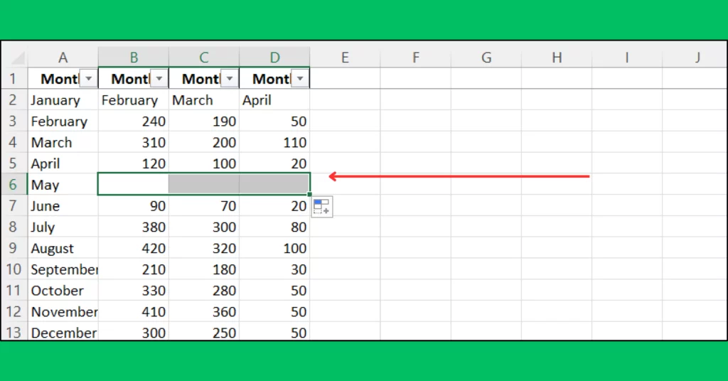
- Remove Blanks: Blank rows or columns can disrupt your data’s flow and make it harder to navigate your spreadsheet efficiently. Remove or fill them before freezing panes.
- Continuous Data: Ensure your data is continuous, as freezing panes work best without interruptions.
5. Decide What to Freeze
- Rows, Columns, or Both: Think about what you constantly need to reference. If it’s the headings, freeze the top row. If it’s row labels, freeze the first column. You might even need to freeze both.
- Test Different Scenarios: Sometimes, it might not be immediately clear what needs to be frozen. Don’t hesitate to try freezing different sections to see what works best for your specific needs.
By taking the time to properly organize and prepare your Excel sheet, you’ll maximize the effectiveness of freezing panes. This preparation ensures that your most crucial data remains in view, facilitating easier navigation and analysis, regardless of the size or complexity of your dataset.
How to Freeze Rows in Excel
Freezing rows in Excel is a straightforward process that can greatly enhance your ability to navigate and analyze your data. Whether you’re working on financial reports, data analysis, or any spreadsheet that requires constant reference to the top rows, these steps will guide you through freezing rows effectively.
Selecting the Row Below the One You Want to Freeze
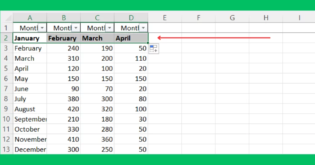
- Decide Which Rows to Keep Visible: First, figure out which rows contain the information you always want to see. This is typically your header row with column titles.
- Select the Row Below: Click on the number to the left of the row that comes right after the last row you want to freeze. For example, if you want to freeze the first two rows, you should click on the row number of the third row. This action highlights the entire row.
Using the View Tab to Freeze Panes
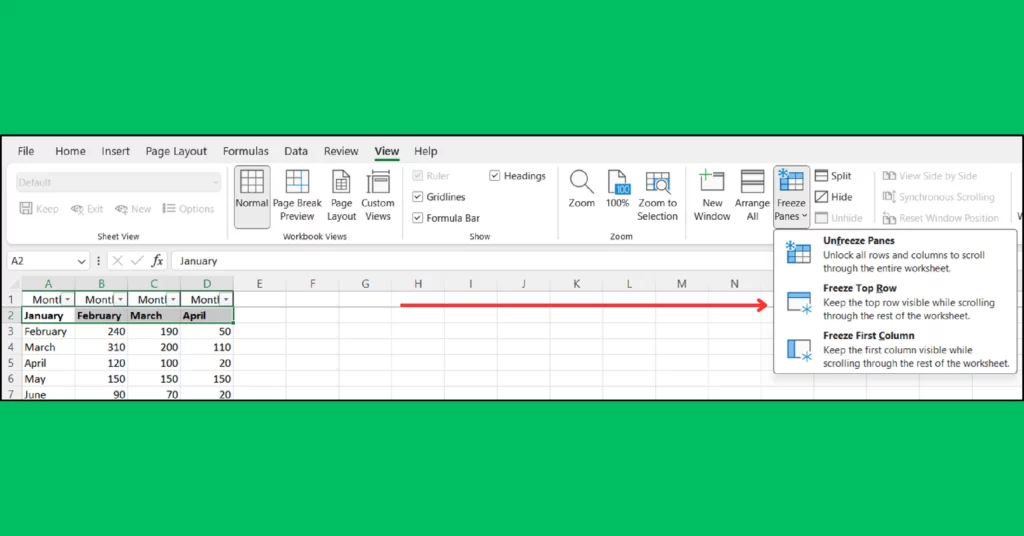
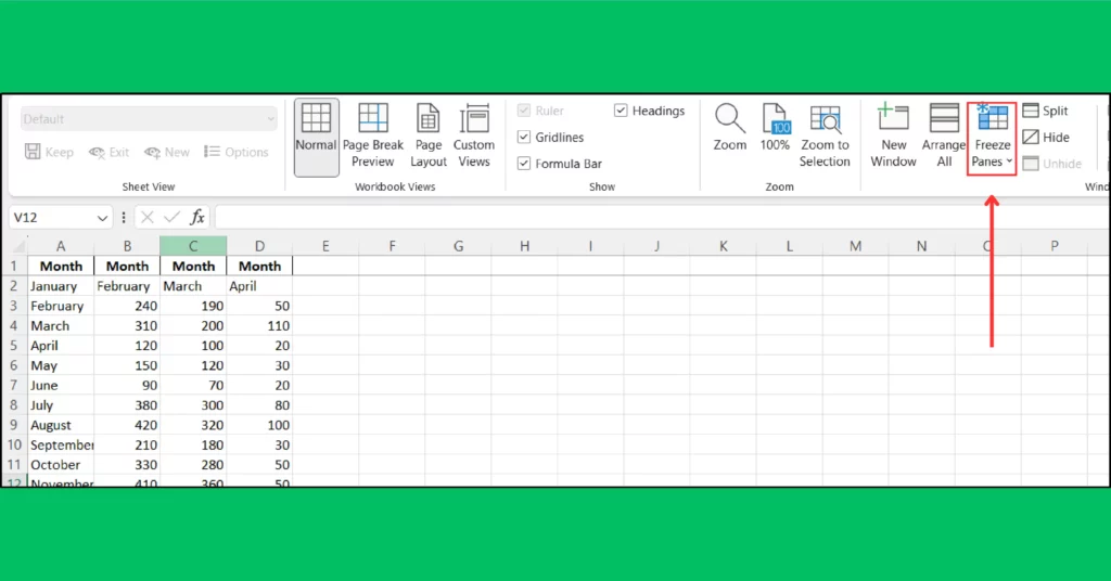
- Navigate to the View Tab: Look at the top of your Excel window to find the ribbon (the toolbar with all the options), and click on the “View” tab. This tab is where you’ll find all the tools related to how you view your spreadsheet.
- Choose Freeze Panes: In the “View” tab, locate the “Freeze Panes” button. You’ll see a small down arrow next to it, which opens up more options when clicked.
- Select Your Freeze Option: Click on “Freeze Panes” from the dropdown menu. Remember, you’ve already selected the row below the ones you want to freeze, so Excel knows to freeze everything above your selected row.
Freezing the Top Row
Sometimes, you may just want to freeze the very top row of your spreadsheet. Here’s how to do it quickly:
- Go to the View Tab: Just like before, find the “View” tab on the ribbon at the top of your Excel window.
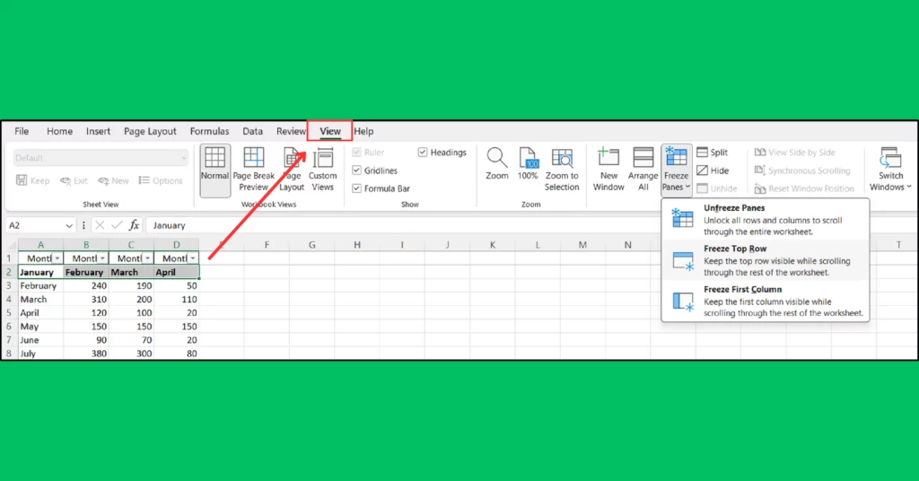
- Click Freeze Panes: Find the “Freeze Panes” button within the “View” tab.
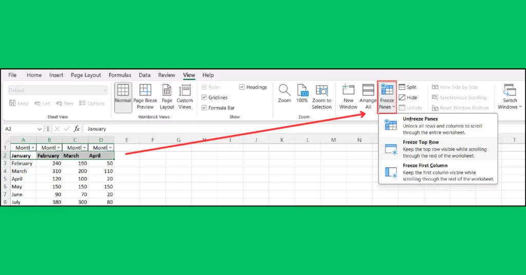
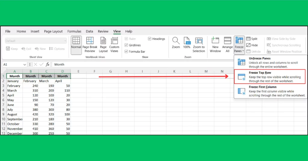
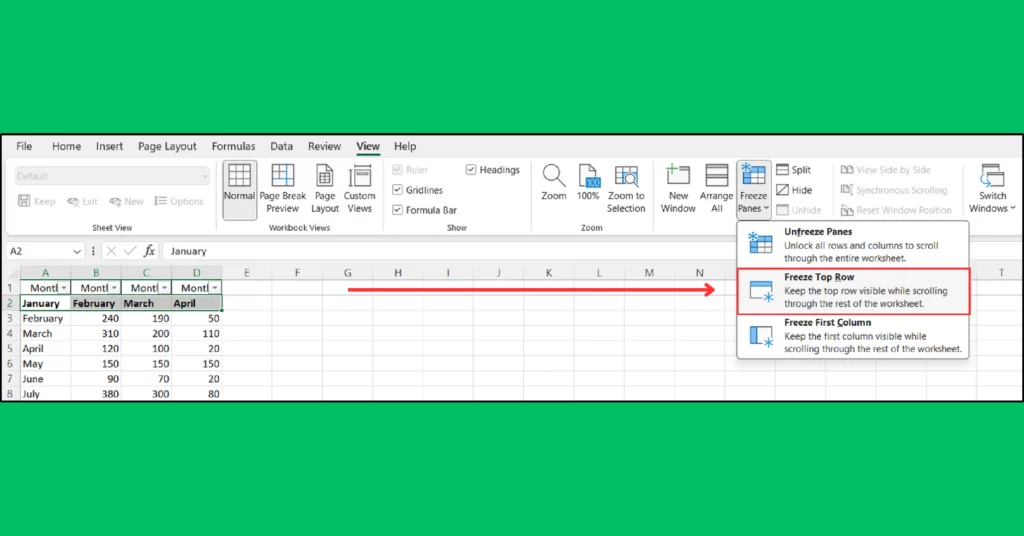
- Choose “Freeze Top Row”: Instead of selecting “Freeze Panes” choose “Freeze Top Row” from the dropdown menu. This option instantly freezes the first row of your spreadsheet, making it always visible as you scroll down.
How to Freeze Columns in Excel
Freezing columns in Excel helps you keep specific sections of your spreadsheet in view while navigating through other parts of your data. This is especially helpful for making sure row names stay in sight. Here’s how to freeze columns effectively:
Selecting the Column to the Right of the One You Want to Freeze
- Identify Columns to Keep Visible: Decide which column(s) contain the essential information you need to keep in view at all times. This is often your first column with row labels or categories.
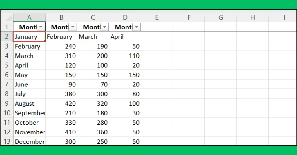
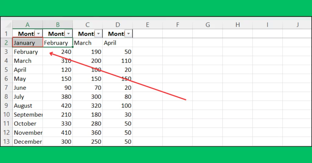
- Select the Next Column: Click on the letter at the top of the column immediately to the right of the last column you want to freeze. For instance, if you want to freeze the first column, you should click on the letter that represents the second column. This highlights the entire column.
Accessing the Freeze Panes Feature
- Open the View Tab: At the top of your Excel window, find the ribbon and click on the “View” tab. This tab contains options related to how you see your spreadsheet.
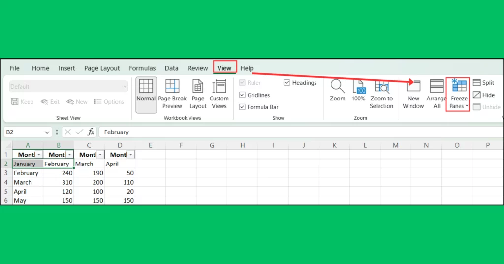
- Locate Freeze Panes: In the “View” tab, find and click on the “Freeze Panes” button. You’ll notice a dropdown arrow next to it, which, when clicked, reveals additional options.
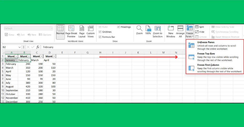
- Use Freeze Panes Option: After clicking “Freeze Panes” from the dropdown list, Excel will freeze everything to the left of the column you selected. This means your chosen columns will remain on the screen as you scroll horizontally.
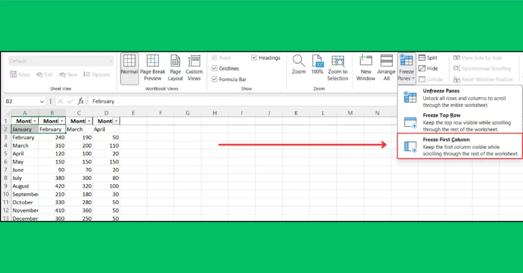
Freezing the First Column
If you only need to keep the first column visible as you scroll through your spreadsheet, follow these simpler steps:
- Navigate to the View Tab: Just as before, go to the ribbon at the top of Excel and click on the “View” tab.

- Click on Freeze Panes: Look for the “Freeze Panes” button within the “View” tab.

- Select “Freeze First Column“: From the dropdown menu, choose “Freeze First Column.” This action immediately freezes the first column of your spreadsheet, ensuring it stays visible no matter how far you scroll to the right.
How to Freeze Both Rows and Columns in Excel
Freezing both rows and columns in Excel allows you to keep crucial headings and row labels visible while you navigate through your spreadsheet. This is particularly useful for large datasets where you need to reference both horizontal and vertical identifiers frequently. Here’s how to do it:
- Decide What to Freeze: First, determine which row and column need to remain in view. Usually, this would be the top row for column headings and the first column for row labels.
- Select the Cell: Click on the cell that is immediately to the right of the column and below the row you want to freeze. For instance, if you want to freeze the first row and the first column, you should select cell B2. This cell’s position tells Excel that you want to freeze everything above and to the left of it.
- Open the View Tab: Go to the top of your Excel window and click on the “View” tab found in the ribbon. This tab contains all the options for how you view your spreadsheet.
- Click on Freeze Panes: In the “View” tab, look for the “Freeze Panes” button. Click the dropdown arrow next to it to reveal more options.
- Select “Freeze Panes” from the Dropdown: Choose the first “Freeze Panes” option from the dropdown list. Unlike the specific “Freeze Top Row” or “Freeze First Column” options, this selection freezes both rows and columns based on the cell you selected in step 2.
How to Unfreeze Panes in Excel
If you’ve previously frozen rows or columns in your Excel spreadsheet and wish to return to a normal view where nothing is frozen, the process is straightforward.
Here’s how you can unfreeze panes:
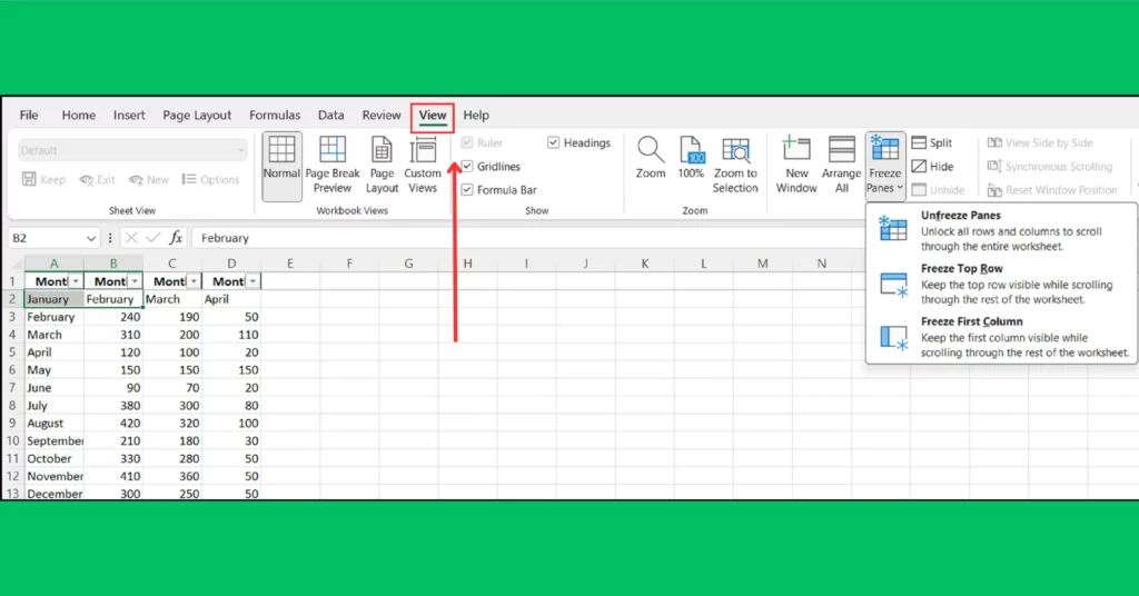
- Go to the View Tab: Start by navigating to the ribbon at the top of your Excel window. Click on the “View” tab, which is where you originally found the options to freeze the panes.
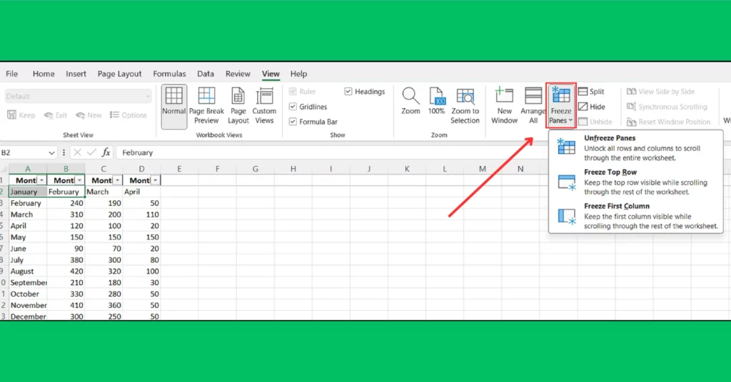
- Find Freeze Panes Button: Within the “View” tab, locate the “Freeze Panes” button. This is the same button you used to freeze panes in the first place.
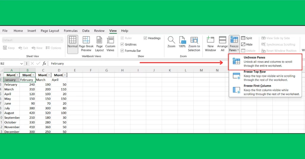
- Select Unfreeze Panes: Click the dropdown arrow next to the “Freeze Panes” button to reveal its options. Here, you’ll see an option labeled “Unfreeze Panes.” Click on this option.
Once you select “Unfreeze Panes” Excel immediately removes any freezing you had on rows, columns, or both. Your spreadsheet will return to its default state, allowing you to scroll freely without any rows or columns remaining fixed on the screen.
This feature is handy for when you’re done analyzing specific parts of your data and want to return to a more flexible view of your spreadsheet. Unfreezing panes is just as simple as freezing them and can be done at any time to adjust your view as needed.
Tips for Effective Data Navigation with Frozen Panes
Using frozen panes wisely in Excel can significantly enhance your data analysis and navigation, especially with large datasets. Here are some tips on making the most out of frozen panes, along with integrating other Excel features for a more powerful data handling experience:
1. Combine Frozen Panes with Filters
- Enhanced Viewing: Apply filters to your columns after freezing panes. This combination allows you to sift through your data without losing sight of your column headers or important row labels, making it easier to perform targeted analysis.
- Dynamic Data Exploration: Use filters to narrow down data, hide irrelevant information, or sort through your dataset while keeping key areas in view.
2. Use Split Screen Alongside Frozen Panes
- Divide Your Workspace: The split screen feature can be used in conjunction with frozen panes for comparing different sections of your spreadsheet. You could freeze the top row or first column and then use a split screen to view and work on distant parts of your data simultaneously.
- Flexible Navigation: This setup provides a more flexible way to navigate large datasets, allowing for side-by-side comparison without losing context.
3. Employ Conditional Formatting
- Visual Cues: With frozen panes, applying conditional formatting helps in highlighting important data points, trends, or anomalies in the visible part of your dataset.
- Immediate Insights: This practice makes it quicker to draw insights from your data, especially when analyzing large datasets with multiple frozen rows or columns.
4. Leverage Excel Tables
- Structured Data: Convert your data range into an Excel table. This gives you the advantage of table functionalities like easy filtering, sorting, and using structured references, which can be particularly beneficial when used in areas outside the frozen panes.
- Integration: Excel tables work well with frozen panes, ensuring that your data is both easy to navigate and manipulate.
Best Practices for Managing Large Datasets with Frozen Panes
- Plan Before You Freeze: Before applying frozen panes, take a moment to plan which rows and columns are most crucial for your analysis. This minimizes the need for frequent adjustments and unfreezing/re-freezing.
- Minimal Freezing: Only freeze what’s necessary. Over-freezing can limit your viewable area, especially on smaller screens, making it harder to work with the rest of your data.
- Use Named Ranges: For large datasets, named ranges can simplify navigation. You can jump to specific data points or sections quickly, complementing the utility of frozen panes.
- Keyboard Shortcuts: Learn and use keyboard shortcuts for freezing and unfreezing panes to speed up your workflow. For example, ALT + W + F can toggle freezing panes on and off, depending on your Excel version and settings.
Also Read:
- How to Create a Drop-Down List in Excel (2024): Discover the steps to easily add a drop-down list to your Excel spreadsheets, enhancing data entry and accuracy.
- How to Clear Cell Contents in Google Sheets: A Step-by-Step Tutorial: Learn the straightforward method for clearing cell contents in Google Sheets, keeping your data organized and up-to-date.
- How to Set Up a Dual Boot for Windows and Linux?: Follow our comprehensive guide on setting up a dual boot system with Windows and Linux, optimizing your computing experience for development and everyday tasks.
Conclusion
Freezing panes in Excel helps you keep important info like titles and labels visible while you scroll through your data. This makes working with big tables much easier because you can always see which data belongs to which column or row.
Quick Tip
Try using freeze panes to see how they help you move around your data better. It’s a simple trick that can make a big difference in how quickly and accurately you can work with lots of information in Excel. The more you use it, the easier it’ll get, so give it a go and see how much smoother your Excel projects can be!


